Bass diffusion model

The Bass model or Bass diffusion model was developed by Frank Bass. It consists of a simple differential equation that describes the process of how new products get adopted in a population. The model presents a rationale of how current adopters and potential adopters of a new product interact. The basic premise of the model is that adopters can be classified as innovators or as imitators, and the speed and timing of adoption depends on their degree of innovation and the degree of imitation among adopters. The Bass model has been widely used in forecasting, especially new products' sales forecasting and technology forecasting. Mathematically, the basic Bass diffusion is a Riccati equation with constant coefficients equivalent to Verhulst—Pearl Logistic growth.

In 1969, Frank Bass published his paper on a new product growth model for consumer durables. Prior to this, Everett Rogers published Diffusion of Innovations, a highly influential work that described the different stages of product adoption. Bass contributed some mathematical ideas to the concept. While the Rogers model describes all four stages of the product lifecycle (Introduction, Growth, Maturity, Decline), The Bass model focuses on the first two (Introduction and Growth). Some of the Bass-Model extensions present mathematical models for the last two (Maturity and Decline).

Model formulation

${\frac {f(t)}{1-F(t)}}=p+qF(t)$

Where:

• $\ F(t)$ is the installed base fraction
• $\ f(t)$ is the rate of change of the installed base fraction, i.e.$\ f(t)=F'(t)$
• $\ p$ is the coefficient of innovation
• $\ q$ is the coefficient of imitation

Expressed as an ordinary differential equation,

${\frac {dF}{dt}}=p(1-F)+q(1-F)F=(1-F)(p+qF).$

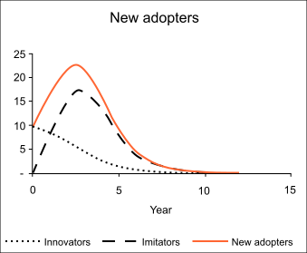
Sales (or new adopters)$\ s(t)$ at time$\ t$ is the rate of change of installed base, i.e.,$\ f(t)$ multiplied by the ultimate market potential$\ m$. Under the condition$\ F(0)=0$, we have that

$\ s(t)=mf(t)$

$\ s(t)=m{\frac {(p+q)^{2}}{p}}{\frac {e^{-(p+q)t}}{(1+{\frac {q}{p}}e^{-(p+q)t})^{2}}}$

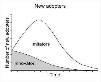
We have the decomposition$\ s(t)=s_{n}(t)+s_{i}(t)$ where$\ s_{n}(t):=mp(1-F(t))$ is the number of innovators at time$\ t$, and$\ s_{i}(t):=mq(1-F(t))F(t)$ is the number of imitators at time$\ t$.

The time of peak sales$\ t^{*}$:

$\ t^{*}={\frac {\ln q-\ln p}{p+q}}$

The times of the inflection points at the new adopters' curve$\ t^{**}$:

$\ t^{**}={\frac {\ln(q/p)-\ln(2\pm {\sqrt {3}}))}{p+q}}$

or in another form (related to peak sales):

$\ t^{**}=t^{*}\pm {\frac {\ln(2+{\sqrt {3}}))}{p+q}}$

The peak time and inflection points' times must be positive. When$\ t^{*}$ is negative, sales have no peak (and decline since introduction). There are cases (depending on the values of$\ p$ and$\ q$) when the new adopters curve (that begins at 0) has only one or zero inflection points.

Explanation

The coefficient$\ p$ is called the coefficient of innovation, external influence or advertising effect. The coefficient$\ q$ is called the coefficient of imitation, internal influence or word-of-mouth effect.

Typical values of$\ p$ and$\ q$ when time$\ t$ is measured in years:

• The average value of$\ p$ has been found to be 0.03, with a typical range between 0.01 and 0.03.
• The average value of$\ q$ has been found to be 0.38, with a typical range between 0.3 and 0.5.

Derivation

The Bass diffusion model is derived by assuming that the hazard rate $\lambda (t)$ for the uptake of a product or service may be defined as:

$$\lambda (t)={f(t) \over {S(t)}}=p+q[1-S(t)]$$

where $f(t)$ is the probability density function and $S(t)=1-F(t)$ is the survival function, with $F(t)$ being the cumulative distribution function. From these basic definitions in survival analysis, we know that:

$$f(t)=-{dS \over {dt}}\implies \lambda (t)=-{1 \over {S}}{dS \over {dt}}$$

Therefore, the differential equation for the survival function is equivalent to:

$${dS \over {S[p+q(1-S)]}}=-dt$$

Integration and rearrangement of terms gives us that:

$${S \over {p+q(1-S)}}=Ae^{-(p+q)t}$$

For any survival function, we must have that $S(0)=1$ and this implies that $A=p^{-1}$. With this condition, the survival function is:

$$S(t)={e^{-(p+q)t}+{q \over {p}}e^{-(p+q)t} \over {1+{q \over {p}}e^{-(p+q)t}}}$$

Finally, using the fact that $F(t)=1-S(t)$, we find that the Bass diffusion model for product uptake is:

$$F(t)={1-e^{-(p+q)t} \over {1+{q \over {p}}e^{-(p+q)t}}}$$

Extensions to the model

Generalised Bass model (with pricing)

Bass found that his model fit the data for almost all product introductions, despite a wide range of managerial decision variables, e.g. pricing and advertising. This means that decision variables can shift the Bass curve in time, but that the shape of the curve is always similar.

Although many extensions of the model have been proposed, only one of these reduces to the Bass model under ordinary circumstances.

This model was developed in 1994 by Frank Bass, Trichy Krishnan and Dipak Jain:

${\frac {f(t)}{1-F(t)}}=(p+{q}F(t))x(t)$

where $\ x(t)$ is a function of percentage change in price and other variables

Unlike the Bass model which has an analytic solution, but can also be solved numerically, the generalized bass models usually do not have analytic solutions and must be solved numerically. Orbach (2016) notes that the values of p,q are not perfectly identical for the continuous-time and discrete-time forms. For the common cases (where p is within the range of 0.01-0.03 and q within the range of 0.2-0.4) the discrete-time and continuous-time forecasts are very close. For other p,q values the forecasts may divert significantly.  

Successive generations

An example of a forecast with 8 generations

Technology products succeed one another in generations. Norton and Bass extended the model in 1987 for sales of products with continuous repeat purchasing. The formulation for three generations is as follows:

$\ S_{1,t}=F(t_{1})m_{1}(1-F(t_{2}))$

$\ S_{2,t}=F(t_{2})(m_{2}+F(t_{1})m_{1})(1-F(t_{3}))$

$\ S_{3,t}=F(t_{3})(m_{3}+F(t_{2})(m_{2}+F(t_{1})m_{1}))$

where

• $\ m_{i}=a_{i}M_{i}$
• $\ M_{i}$ is the incremental number of ultimate adopters of the ith generation product
• $\ a_{i}$ is the average (continuous) repeat buying rate among adopters of the ith generation product
• $\ t_{i}$ is the time since the introduction of the ith generation product
• $\ F(t_{i})={\frac {1-e^{-(p+q)t_{i}}}{1+{\frac {q}{p}}e^{-(p+q)t_{i}}}}$

It has been found that the p and q terms are generally the same between successive generations.

Relationship with other s-curves

There are two special cases of the Bass diffusion model.

• The first special case occurs when q=0, when the model reduces to the exponential distribution.
• The second special case reduces to the logistic distribution, when p=0.

The Bass model is a special case of the Gamma/shifted Gompertz distribution (G/SG): Bemmaor (1994)

Use in online social networks

The rapid, recent (as of early 2007) growth in online social networks (and other virtual communities) has led to an increased use of the Bass diffusion model. The Bass diffusion model is used to estimate the size and growth rate of these social networks. The work by Christian Bauckhage and co-authors shows that the Bass model provides a more pessimistic picture of the future than alternative model(s) such as the Weibull distribution and the shifted Gompertz distribution.

The ranges of the p, q parameters

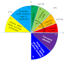
Bass (1969) distinguished between a case of p<q wherein periodic sales grow and then decline (a successful product has a periodic sales peak); and a case of p>q wherein periodic sales decline from launch (no peak).

Jain et al. (1995) explored the impact of seeding. When using seeding, diffusion can begin when p + qF(0) > 0 even if p’s value is negative, but a marketer uses seeding strategy with seed size of F(0) > -p/q . The interpretation of a negative p value does not necessarily mean that the product is useless: There can be cases wherein there are price or effort barriers to adoption when very few others have already adopted. When others adopt, the benefits from the product increase, due to externalities or uncertainty reduction, and the product becomes more and more plausible for many potential customers.

Moldovan and Goldenberg (2004) incorporated negative word of mouth (WOM) effect on the diffusion, which implies a possibility of a negative q. Negative q does not necessarily mean that adopters are disappointed and dissatisfied with their purchase. It can fit a case wherein the benefit from a product declines as more people adopt. For example, for a certain demand level for train commuting, reserved tickets may be sold to those who like to guarantee a seat. Those who do not reserve seating may have to commute while standing. As more reserved seating are sold, the crowding in the non-reserved railroad car is reduced, and the likelihood of finding a seat in the non-reserved car increases, thus reducing the incentive to buy reserved seating. While the non-cumulative sales curve with negative q is similar to those with q=0, the cumulative sales curve presents a more interesting situation: When p > -q, the market will reach 100% of its potential, eventually, as for a regular positive value of q. However, if p < -q, at the long-range, the market will saturate at an equilibrium level –p/q of its potential.

Orbach (2022) summarized the diffusion behavior at each portion of the p,q space and maps the extended (p,q) regions beyond the positive right quadrant (where diffusion is spontaneous) to other regions where diffusion faces barriers (negative p), where diffusion requires “stimuli” to start, or resistance of adopters to new members (negative q), which might stabilize the market below full adoption, occur.

A map of the extended Bass p-q space

Adoption of this model

The model is one of the most cited empirical generalizations in marketing; as of August 2023 the paper "A New Product Growth for Model Consumer Durables" published in Management Science had (approximately) 11352 citations in Google Scholar.

This model has been widely influential in marketing and management science. In 2004 it was selected as one of the ten most frequently cited papers in the 50-year history of Management Science. It was ranked number five, and the only marketing paper in the list. It was subsequently reprinted in the December 2004 issue of Management Science.

The Bass model was developed for consumer durables. However, it has been used also to forecast market acceptance of numerous consumer and industrial products and services, including tangible, non-tangible, medical, and financial products. Sultan et al. (1990) applied the Bass model to 213 product categories, mostly consumer durables (in a wide range of prices) but also to services such as motels and industrial/farming products like hybrid corn seeds.

See also

• Diffusion of innovation
• Forecasting
• Lazy user model
• Shifted Gompertz distribution