
File:Comparison of symmetric and periodic triangular window functions.svg

Size of this PNG preview of this SVG file: 511 × 600 pixels. Other resolutions: 204 × 240 pixels | 409 × 480 pixels | 654 × 768 pixels | 873 × 1,024 pixels | 1,745 × 2,048 pixels | 652 × 765 pixels.
Original file (SVG file, nominally 652 × 765 pixels, file size: 94 KB)
| This is a file from the Wikimedia Commons. Information from its description page there is shown below. Commons is a freely licensed media file repository. You can help. |
Summary
| Description |
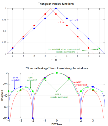
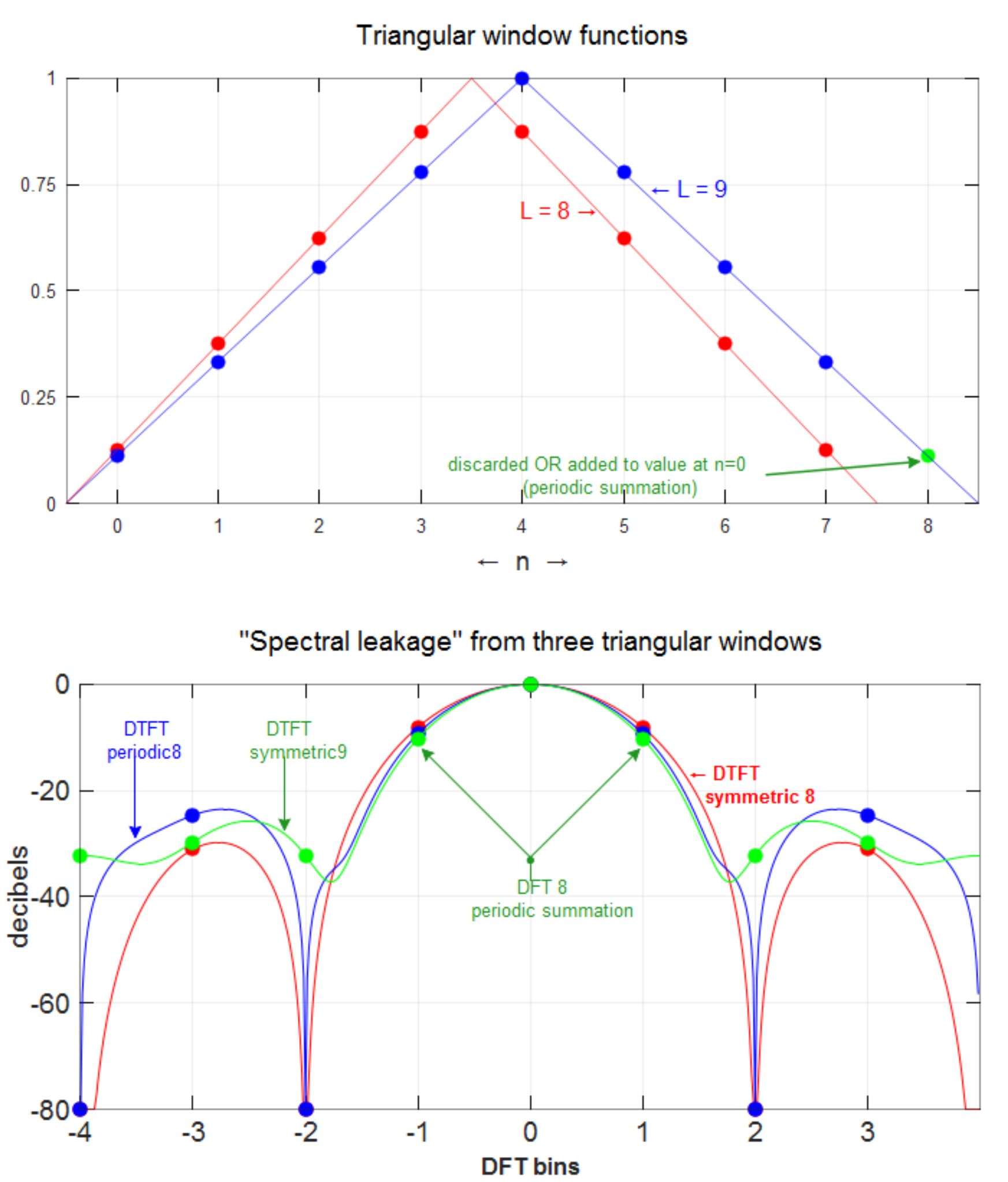
English: These figures compare two 8-length triangle window functions and their spectral leakage (discrete-time Fourier transform) characteristics. The function labeled DFT-even is a truncated version of a 9-length symmetric window, whose DTFT is also shown (in green). All three DTFTs have been sampled at the same frequency interval (by an 8-length DFT). In the case of the 9-length window, that is done by combining its first and last coefficients by addition (called periodic summation, with period 8). Because of symmetry, those coefficients are equal. So in a spectral analysis (of data) application, an equivalent operation is to add the 9th data sample to the 1st one, and apply the same 8-length DFT-even window function seen in the top figure. |
|||
| Date | ||||
| Source | Own work | |||
| Author | Bob K | |||
| Permission (Reusing this file) |
I, the copyright holder of this work, hereby publish it under the following license:
|
|||
| Other versions |
This file was derived from: 8-point windows.gif |
|||
| SVG development | This W3C-invalid vector image was created with LibreOffice. |
|||
| Gnu Octave source | click to expand
This graphic was created with the help of the following Octave script: graphics_toolkit gnuplot
pkg load signal
darkgreen = [33 150 33]/256;
M=7200; % big number, divisible by 8 and 9
% Generate M+1 samples of a triangle window
window = triang(M+1)'; % row vector
N=8; % actual window size, in "hops"
% Sample the triangle.
% Scale the abscissa. 0:M samples --> 0:9 "hops", and take 9 symmetrical hops, from .5 to 8.5
sam_per_hop_9 = M/9;
symmetric9 = window(1+(.5:8.5)*sam_per_hop_9);
periodic8 = symmetric9(1:8);
periodic_summation = [symmetric9(1)+symmetric9(N+1) symmetric9(2:N)];
% Re-scale the abscissa. 0:M samples --> 0:8 "hops", and take 8 symmetrical hops, from .5 to 7.5
sam_per_hop_8 = M/8;
symmetric8 = window(1+(.5:7.5)*sam_per_hop_8);
%------------------------------------------------------------------
% Compare windows based on their processing gain (PG) (Harris,1978,p 56,eq 15), because the ENBW
% formula allows values less than one "bin" (for some windows) when used with a 9-point periodic
% summation and an 8-point DFT. That actually makes sense, because a bandwidth of 1.1 (for instance)
% measured in 1/9-width bins is only 0.98 measured in 1/8-width bins. But values less than one
% are not customary, which could cause distrust.
PG_symmetric8 = sum(symmetric8)^2/sum(symmetric8.^2) % 6.0968
PG_periodic8 = sum(periodic8)^2 /sum(periodic8.^2) % 6.4529
PG_symmetric9 = sum(symmetric9)^2/sum(symmetric9.^2) % 6.7529
% Also note that the correct incoherent "power" formula for the
% periodic_summation window is sum(symmetric9.^2),
% not sum(periodic_summation.^2), because
% E{(h(1)·X(1) + h(9)·X(9))^2} = (h(1)^2 + h(9)^2)·E{X^2},
% not (h(1)^2 + 2·h(1)·h(9) + h(9)^2)·E{X^2}.
%------------------------------------------------------------------
% Plot the points
figure("position", [1 1 700 400])
plot(0:7, symmetric8, "color","red", ".", "markersize",14)
hold on
plot(8, symmetric9(9), "color","green", ".", "markersize",14)
plot(0:7, periodic8, "color","blue", ".", "markersize",14)
% Connect the dots
hops = (0:M)/sam_per_hop_9 -.5;
plot(hops, window, "color","blue") % periodic
hops = (0:M)/sam_per_hop_8 -.5;
plot(hops, window, "color","red") % symmetric
xlim([-.5 8.5])
set(gca, "xgrid","on")
set(gca, "ygrid","on")
set(gca, "ytick",[0:.25:1])
set(gca, "xtick",[0:8])
text(3.98, 0.69, 'L = 8 \rightarrow', "color","red", "fontsize",12)
text(5.25, 0.74, '\leftarrow L = 9', "color","blue", "fontsize",12)
title("Triangular window functions", "fontsize",14, "fontweight","normal")
xlabel('\leftarrow n \rightarrow', "fontsize",14)
% After this call, the cursor units change to a normalized ([0,1]) coordinate system
annotation("textarrow", [.76 .911], [.177 .2], "color",darkgreen,...
"string",{"discarded OR added to value at n=0 ";...
" (periodic summation)"}, "fontsize",10,...
"linewidth",1.5, "headstyle","vback1", "headlength",5, "headwidth",5)
%Now compute and plot the DTFTs and DFTs
M=64*N; % DTFT size
dr = 80; % dynamic range (decibels)
%------------------------------------------------------------------
% DTFT of symmetric window
H = abs(fft([symmetric8 zeros(1,M-N)]));
H = fftshift(H);
H = H/max(H);
H = 20*log10(H);
H = max(-dr,H);
x = N*[-M/2:M/2-1]/M;
figure("position", [1 1 700 400])
plot(x, H, "color","red", "linewidth",1);
hold on
ylim([-dr 0])
% Compute a DFT to sample the DTFT 8 times
H = abs(fft(symmetric8));
H = fftshift(H);
H = H/max(H);
H = 20*log10(H);
H = max(-dr,H);
plot(-N/2:(N/2-1), H, "color","red", ".", "markersize",14)
%------------------------------------------------------------------
% DTFT of periodic window
H = abs(fft([periodic8 zeros(1,M-N)]));
H = fftshift(H);
H = H/max(H);
H = 20*log10(H);
H = max(-dr,H);
plot(x, H, "color","blue", "linewidth",1);
% Compute a DFT to sample the DTFT 8 times
H = abs(real(fft(periodic8))); % real() is redundant... just to illustrate a point
H = fftshift(H);
H = H/max(H);
H = 20*log10(H);
H = max(-dr,H);
plot(-N/2:(N/2-1), H, "color","blue", ".", "markersize",14)
%------------------------------------------------------------------
% DTFT of a 9-sample symmetric window
H = abs(fft([symmetric9 zeros(1,M-N-1)]));
H = fftshift(H);
H = H/max(H);
H = 20*log10(H);
H = max(-dr,H);
plot(x, H, "color","green", "linewidth",1);
% Compute a DFT to sample the DTFT only 8 times.
H = abs(real(fft(periodic_summation))); % real() is redundant... just to illustrate a point
H = fftshift(H);
H = H/max(H);
H = 20*log10(H);
H = max(-dr,H);
plot(-N/2:(N/2-1), H, "color","green", ".", "markersize",14)
set(gca,"XTick", -N/2:N/2-1)
grid on
text(1.41, -18.8, {'\leftarrow DTFT';" symmetric 8"}, "color","red",...
"fontsize",10, "fontweight","bold")
set(gca,"XTick", -N/2:N/2-1)
grid on
ylabel("decibels", "fontsize",14)
xlabel("DFT bins", "fontsize",12, "fontweight","bold")
title('"Spectral leakage" from three triangular windows', "fontsize",14, "fontweight","normal")
% After this call, the cursor units change to a normalized ([0,1]) coordinate system
annotation("textarrow", [.132 .132], [.74 .6],...
"color", "blue", "string", {" DTFT";"periodic8"}, "fontsize",10,...
"linewidth",1, "headstyle","vback1", "headlength",5, "headwidth",5)
annotation("textarrow", [.28 .28], [.74 .613],...
"color", darkgreen, "string", {" DTFT";"symmetric9"}, "fontsize",10,...
"linewidth",1, "headstyle","vback1", "headlength",5, "headwidth",5)
annotation("arrow", [.524 .417], [.565 .752],...
"color", darkgreen,...
"linewidth",1, "headstyle","vback1", "headlength",5, "headwidth",5)
annotation("arrow", [.524 .632], [.565 .752],...
"color", darkgreen,...
"linewidth",1, "headstyle","vback1", "headlength",5, "headwidth",5)
annotation("textarrow", [.524 .524], [.525 .565], "color",darkgreen, "fontsize",10,...
"string",{" DFT 8";"periodic summation"},...
"linewidth",1, "headstyle","ellipse", "headlength",3, "headwidth",3)
% annotation("arrow", [.524 .311], [.565 .565], "linestyle", "--",...
% "color", darkgreen,...
% "linewidth",1, "headstyle","vback1", "headlength",5, "headwidth",5)
% annotation("arrow", [.524 .738], [.565 .565], "linestyle", "--",...
% "color", darkgreen,...
% "linewidth",1, "headstyle","vback1", "headlength",5, "headwidth",5)
|
File history
Click on a date/time to view the file as it appeared at that time.
| Date/Time | Thumbnail | Dimensions | User | Comment | |
|---|---|---|---|---|---|
| current | 21:49, 31 March 2020 | | 652 × 765 (94 KB) | Bob K | Remove legend from 2nd image, because: The equivalent noise bandwidth formula allows values less than one "bin" (for some windows) when used with a 9-point periodic summation and an 8-point DFT. That actually makes sense, because a bandwidth of 1.1 (for instance) measured in 1/9-width bins is only 0.98 measured in 1/8-width bins. But values less than one are not customary. |
| 15:33, 30 September 2019 |  | 652 × 765 (101 KB) | Bob K | add a label to the legend in figure #2 | |
| 15:01, 21 March 2019 |  | 652 × 765 (100 KB) | Bob K | move a label on graph #2 | |
| 12:21, 20 March 2019 |  | 652 × 765 (98 KB) | Bob K | replace a missing label on the lower graph | |
| 20:51, 17 March 2019 |  | 652 × 765 (97 KB) | Bob K | Declutter. | |
| 16:24, 13 March 2019 |  | 652 × 765 (101 KB) | Bob K | Larger canvas. Better annotations. Replace "folding" with "circular addition" and "periodic summation". | |
| 23:44, 12 March 2019 |  | 522 × 630 (74 KB) | Bob K | User created page with UploadWizard |
File usage
No pages on the English Wikipedia use this file (pages on other projects are not listed).