
File:Helmholtz solution.png

Size of this preview: 298 × 598 pixels. Other resolutions: 119 × 240 pixels | 239 × 480 pixels | 975 × 1,957 pixels.
Original file (975 × 1,957 pixels, file size: 23 KB, MIME type: image/png)
| This is a file from the Wikimedia Commons. Information from its description page there is shown below. Commons is a freely licensed media file repository. You can help. |
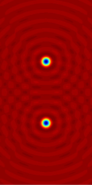
| Description | Illustration of en:Helmholtz equation. |
| Date | (UTC) |
| Source | self-made with en:Matlab. See the source code below. |
| Author | Oleg Alexandrov |
This diagram was created with MATLAB.
| I, the copyright holder of this work, release this work into the public domain. This applies worldwide. In some countries this may not be legally possible; if so: I grant anyone the right to use this work for any purpose, without any conditions, unless such conditions are required by law. |
Source code (MATLAB)
% Plot the solution to the Helmholtz equation with a given source
clear all;

Box_x = 3;
Scale = 0.5;
Box_y = Box_x/Scale;

Nx = 200;
Ny = Nx/Scale;

wavenumber = 10;

XX = linspace(-Box_x, Box_x, Nx);
YY = linspace(-Box_y, Box_y, Ny);
hx = XX(2) - XX(1);
hy = YY(2) - YY(1);
[X, Y] = meshgrid(XX, YY);

Source_size  = 0.5;
Source_shift = 2;
Source =  max(Source_size^2 - X.^2-(Y-Source_shift).^2, 0) + max(Source_size^2 - X.^2-(Y+Source_shift).^2, 0) ;

% plot the source
figure(1); clf; hold on; axis equal; axis off;
imagesc(Source);


% plot the solution to the Helmholtz equation
I = sqrt(-1);
Field = 0*X;

[m, n] = size(Source);
for i=1:m
   i
   for j=1:n

      if Source(i, j) ~= 0

	 x0 = X(i, j);
	 y0 = Y(i, j);

	 % add the contribution from the current source
	 Field = Field + (I/4)*besselh(0, 1, wavenumber*sqrt((X-x0).^2+(Y-y0).^2) + eps)*Source(i, j)*hx*hy;
      end

   end
end


figure(2); clf; hold on; axis equal; axis off;
imagesc(real(Field));

% Save to disk and convert to png right away
figure(1);
saveas(gcf, 'Helmholtz_source.eps', 'psc2');
%! convert -density 200 Helmholtz_source.eps Helmholtz_source.png

figure(2);
saveas(gcf, 'Helmholtz_solution.eps', 'psc2');
%! convert -density 200 Helmholtz_solution.eps Helmholtz_solution.png

|
This math image could be re-created using vector graphics as an SVG file. This has several advantages; see Commons:Media for cleanup for more information. If an SVG form of this image is available, please upload it and afterwards replace this template with
{{vector version available|new image name}}.
It is recommended to name the SVG file “Helmholtz solution.svg”—then the template Vector version available (or Vva) does not need the new image name parameter. |
File history
Click on a date/time to view the file as it appeared at that time.
| Date/Time | Thumbnail | Dimensions | User | Comment | |
|---|---|---|---|---|---|
| current | 19:50, 7 July 2007 | | 975 × 1,957 (23 KB) | Oleg Alexandrov | Tweak |
| 04:18, 7 July 2007 |  | 500 × 989 (22 KB) | Oleg Alexandrov | Higher res. | |
| 03:59, 7 July 2007 |  | 500 × 989 (15 KB) | Oleg Alexandrov | {{Information |Description=Illustration of en:Helmholtz equation. |Source=self-made with en:Matlab. See the source code below. |Date=03:56, 7 July 2007 (UTC) |Author= Oleg Alexandrov }} {{PD-self}} ==MATLAB source code |
File usage
The following pages on the English Wikipedia use this file (pages on other projects are not listed):
Global file usage
The following other wikis use this file:
- Usage on ar.wikipedia.org
- Usage on ca.wikipedia.org
- Usage on et.wikipedia.org
- Usage on fa.wikipedia.org
- Usage on fr.wikipedia.org
- Usage on ko.wikipedia.org
- Usage on no.wikipedia.org
- Usage on pt.wikipedia.org
- Usage on sq.wikipedia.org
- Usage on vi.wikipedia.org
- Usage on www.wikidata.org
- Usage on zh.wikipedia.org