
File:US polls 2016.svg

Size of this PNG preview of this SVG file: 800 × 444 pixels. Other resolutions: 320 × 178 pixels | 640 × 356 pixels | 1,024 × 569 pixels | 1,280 × 711 pixels | 2,560 × 1,422 pixels | 810 × 450 pixels.
Original file (SVG file, nominally 810 × 450 pixels, file size: 180 KB)
| This is a file from the Wikimedia Commons. Information from its description page there is shown below. Commons is a freely licensed media file repository. You can help. |
Summary
| Description |
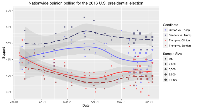
English: A combination of nationwide opinion polls during the 2016 U.S. presidential election. The trend lines are Local Regressions with α = 0.8 and 95% confidence interval ribbons. The point sizes and trend lines are weighted according to the margin of error of each poll. |
| Date | |
| Source | Own work |
| Author | Abjiklam |
Licensing
I, the copyright holder of this work, hereby publish it under the following license:
This file is licensed under the Creative Commons Attribution-Share Alike 4.0 International license.
- You are free:
- to share – to copy, distribute and transmit the work
- to remix – to adapt the work
- Under the following conditions:
- attribution – You must give appropriate credit, provide a link to the license, and indicate if changes were made. You may do so in any reasonable manner, but not in any way that suggests the licensor endorses you or your use.
- share alike – If you remix, transform, or build upon the material, you must distribute your contributions under the same or compatible license as the original.
Code
The graph is generated by the following R script, largely inspired by this file.
library(RCurl)
library(reshape)
library(htmltab)
library(ggplot2)
library(stringr)
library(scales)

#get the table from the url
theurl <- getURL("https://en.wikipedia.org/wiki/Nationwide_opinion_polling_for_the_United_States_presidential_election,_2016", ssl.verifyPeer=FALSE)
table <- htmltab(theurl, which=3)

df = table[, c(2, 8, 3:6)]

names(df) <- c("Date", "Size", "DC", "DP", "RC", "RP")

df = df[which(df$RC=="Donald Trump"), ]
df[which(df$DC=="Bernie Sanders"), ]$DC = "Sanders"
df[which(df$DC=="Hillary Clinton"), ]$DC = "Clinton"
df[which(df$RC=="Donald Trump"), ]$RC = "Trump"
df[which(df$DC=="Sanders" & df$RC=="Trump"), ]$RC = "Trump2"

df$Contest = paste(substr(df$DC, 1, 1), substr(df$RC, 1, 1))

dem.df = df[, c(1:4, 7)]
rep.df = df[, c(1:2, 5:7)]

names(dem.df)[3:4] <- c("Candidate", "Support")
names(rep.df) <- names(dem.df)

df = rbind(dem.df, rep.df)

df$Support = as.numeric(sub("%", "", df$Support))/100

df$Date = sub("[0-9]+\\s*–\\s*([0-9]+)", "\\1", df$Date)
df$Date = sub(".*–", "", df$Date)
df$Date = sub("[0-9]+\\s*-\\s*([0-9]+)", "\\1", df$Date)
df$Date = sub(".*-", "", df$Date)
df$Date = trimws(df$Date)
df$Date = as.Date(df$Date, format="%B %d, %Y")

df$Size = as.numeric(sub(",", "", df$Size))

df$Error = 1/sqrt(df$Size)

cols = c("#6666FF", "#333366", "#FF3333", "#993333")
labs = c("Clinton vs. Trump", "Sanders vs. Trump", "Trump vs. Clinton", "Trump vs. Sanders")

results = df

#breaks() returns n evenly spaced numbers between x and y
#whose squares are divisible by p
#the function is used for the legend
breaks <- function(x, y, n, p) {
  x = sqrt(ceiling(as.integer(x^2) / p) * p)
  y = sqrt(floor(as.integer(y^2) / p) * p)
  s = seq(x, y, length.out=n)
  for (i in 2:(n-1)) {
    s[i] = sqrt(round(s[i]^2 / p) * p)
  }
  return(unique(s))
}

d = ggplot(results, aes(x=Date, y=Support,
                        colour=Candidate, linetype=Candidate, shape=Candidate,
                        size=1/Error, weight=1/Error)) +
  labs(title="Nationwide opinion polling for the 2016 U.S. presidential election") +
  geom_point(alpha=0.7) +
  geom_smooth(span=0.8, show.legend=F, alpha=0.2) +
  scale_colour_manual(name="Candidate", values=cols, labels=labs) +
  scale_shape_manual(name="Candidate", values=c(16, 15, 16, 15), labels=labs) +
  scale_linetype_manual(name="Candidate", values=c(1, 5, 1, 5), labels=labs) +
  scale_size_area(max_size=3,
                  breaks=function(x) breaks(x[1], x[2], 5, 100), #5 numbers divisible by 100
                  labels=function(x) comma_format()(x^2),
                  name="Sample Size") +
  scale_y_continuous(breaks=seq(0,1,0.05), minor_breaks=seq(0,1,0.01), labels=percent,
                     limits=c(0.34, 0.6)) +
  scale_x_date(labels=date_format("%b %d"),
               breaks=sort(c(seq(as.Date("2016/1/1"), as.Date("2016/10/1"), "month"),
                             as.Date("2016/11/8")))) +
  theme(panel.grid.minor=element_line(size=0.2),
        panel.grid.major=element_line(size=0.6))

#save plot as "us2016.svg"
svg(filename="us2016.svg",
    width=9,
    height=5,
    pointsize=12,
    bg="transparent")
d
dev.off()
File history
Click on a date/time to view the file as it appeared at that time.
| Date/Time | Thumbnail | Dimensions | User | Comment | |
|---|---|---|---|---|---|
| current | 14:06, 8 June 2016 | | 810 × 450 (180 KB) | Χ | update |
| 01:38, 7 June 2016 |  | 810 × 360 (178 KB) | Χ | update | |
| 17:33, 2 June 2016 |  | 810 × 360 (177 KB) | Χ | update | |
| 00:49, 2 June 2016 |  | 810 × 360 (175 KB) | Χ | User created page with UploadWizard |
File usage
The following page uses this file: