THIS IS A ROUGH DRAFT, NEEDS A LOT OF WORK
Helmert's distribution of sn
[edit]The distribution of the sample standard deviation sn was derived by Helmert [1], and is given by
![{\displaystyle s_{n}\,\,\sim \,\,\,{{n^{{n-1} \over 2}} \over {2^{{n-3} \over 2}\,\,\Gamma \left({{n-1} \over 2}\right)\,\,\sigma ^{n-1}}}\,\,\,\,s_{n}^{n-2}\,\,\exp \left[{{-n\,s_{n}^{2}} \over {2\,\sigma ^{2}}}\right]}](https://wikimedia.org/api/rest_v1/media/math/render/svg/f6a92d4664ee21e82327443329fe4125df858655)
where n is the sample size, taken from an NID population whose true standard deviation is σ. The statistic sn is found using

as opposed to the statistic sn−1 as defined above, in which the divisor under the square root is n−1. It can be shown [2] that the expected value (mean) of this distribution is
![{\displaystyle {\rm {E}}\left[{s_{n}}\right]\,\,\,=\,\,\,\sigma \,\,\left\{{{\sqrt {{2\pi } \over n}}\,\,{1 \over {B\left({{{n-1} \over 2},{1 \over 2}}\right)}}}\right\}}](https://wikimedia.org/api/rest_v1/media/math/render/svg/34c415997d43e73096d5a0b1618811e061d02c18)
where B( ) is the beta function. Using an identity for the beta and gamma functions[3]

it follows that
![{\displaystyle {\rm {E}}\left[{s_{n}}\right]\,\,\,=\,\,\,\sigma \,\,{\sqrt {\,{2 \over n}}}\,\,\,{{\Gamma \left({n \over 2}\right)} \over {\Gamma \left({{n-1} \over 2}\right)}}\,\,\,\,\,=\,\,\,\sigma \,c_{2}}](https://wikimedia.org/api/rest_v1/media/math/render/svg/09359d03f0e66bc94a94c88e2bec3ddf0bc0e4fb)
The symbol c2 is used in quality control [4]. In fact, the rth moment of this PDF can be found using[5]
![{\displaystyle {\rm {E}}\left[{s_{n}^{\,\,r}}\right]\,\,\,=\,\,\,\,\sigma ^{r}\,\,\left({2 \over n}\right)^{r \over 2}\,\,{{\,\Gamma \left({{n+\,\,r-1} \over 2}\right)} \over {\Gamma \left({{n-1} \over 2}\right)}}}](https://wikimedia.org/api/rest_v1/media/math/render/svg/8191ba913d61ede92216f790cca79071ba2b478a)
Using series expansions, it can be shown that an approximate value for c2 can be obtained from[6]

Distribution of normalized sn
[edit]It is useful to have the PDF of the ratio of sn to σ so that plots, for example, will be scale-independent. This amounts to a simple change of variable in the Helmert distribution. Since σ is a constant, it is straightforward to show that[7]
![{\displaystyle {{s_{n}} \over \sigma }\,\,\,\sim \,\,\,{{n^{{n\,-\,1} \over 2}} \over {2^{{n\,-\,3} \over 2}\,\,\,\Gamma \left({{n-1} \over 2}\right)}}\,\,\,\left({{s_{n}} \over \sigma }\right)^{n-2}\exp \left[{-\,\,{n \over 2}\left({{s_{n}} \over \sigma }\right)^{2}}\right]}](https://wikimedia.org/api/rest_v1/media/math/render/svg/5238c7e0a902faed9083e8979d7f3d502c0f1778)
and the expected value (mean) of this PDF is
![{\displaystyle {\rm {E}}\left[{{s_{n}} \over \sigma }\right]\,\,\,=\,\,\,c_{2}}](https://wikimedia.org/api/rest_v1/media/math/render/svg/e102429bc100884aa7a0ddbd14c8bcb03c9d0fde)
To illustrate this PDF, consider Figure 1 (the figures are in a gallery at the bottom of the article). This shows the Helmert PDF (solid line) and a histogram of 10000 sampled sn values, both normalized to the known standard deviation of the NID population. The vertical dashed line, just visible near the solid line showing the location of c2, is the location of the observed mean of these sn values. (The circles plotted on this figure will be addressed below.) Clearly the histogram and the PDF, and the observed mean and c2 agree well.
Figure 2 shows the behavior of the PDF of the normalized sn as the sample size increases. The c2 values, which are the means of the respective PDFs, are indicated. (The c2 for n=2 is the leftmost thin vertical line.)
Distribution of normalized sn−1
[edit]Since it is the case that

then

and everything in the parentheses is a constant. Returning to the Helmert PDF and again using the change-of-variable calculations, the result is
![{\displaystyle {{s_{n-1}} \over \sigma }\,\,\,\sim \,\,\,{{\left({n-1}\right)^{{n\,-\,1} \over 2}} \over {2^{{n\,-\,3} \over 2}\,\,\Gamma \left({{n-1} \over 2}\right)}}\,\,\,\left({{s_{n-1}} \over \sigma }\right)^{n-2}\exp \left[{-\,\,{{n-1} \over 2}\left({{s_{n-1}} \over \sigma }\right)^{2}}\right]}](https://wikimedia.org/api/rest_v1/media/math/render/svg/fe4803528573bbe349ba96fdc753175433e62ac7)
The expected value is[8]
![{\displaystyle {\rm {E}}\left[{s_{n-1}}\right]\,\,\,=\,\,\,\sigma \,\,{\sqrt {\,{2 \over {n\,\,-1}}}}\,\,\,{{\Gamma \left({n \over 2}\right)} \over {\Gamma \left({{n-1} \over 2}\right)}}\,\,\,=\,\,\,\sigma \,c_{4}\,\,\,\,\,\,\,\,\Rightarrow \,\,\,\,\,\,\,\,{\rm {E}}\left[{{s_{n-1}} \over \sigma }\right]\,\,\,=\,\,c_{4}}](https://wikimedia.org/api/rest_v1/media/math/render/svg/8d79603a6bfafaa369e623ce2a857b604eb1d50d)
where c4 again is a statistical quality control symbol; its series approximation is

Simulation results for the sn−1 case are shown in Figures 3 and 4.
Relation of Helmert to Chi distribution
[edit]The Chi PDF [9] is
![{\displaystyle \chi \,\,\,\sim \,\,\,{1 \over {2^{{k \over 2}\,\,-\,\,1}\,\,\,\Gamma \left({k \over 2}\right)}}\,\,\,\chi ^{k\,-\,1}\,\,\,\exp \left[{{-\chi ^{2}} \over 2}\right]}](https://wikimedia.org/api/rest_v1/media/math/render/svg/2d7822c2747eded456dfcc7a677b3f9287fab2bf)
where k is the number of degrees of freedom. Taking k = n − 1, making the substitution

and using the change-of-variable calculations once again,
![{\displaystyle {{s_{n}} \over \sigma }\,\,\,\sim \,\,\,{1 \over {2^{{n\,-\,3} \over 2}\,\,\Gamma \left({{n-1} \over 2}\right)}}\,\,\,\left({{{\sqrt {n}}\,s_{n}} \over \sigma }\right)^{n-2}\exp \left[{-{1 \over 2}\left({{{\sqrt {n}}\,s_{n}} \over \sigma }\right)^{2}}\right]\left({\sqrt {n}}\right)}](https://wikimedia.org/api/rest_v1/media/math/render/svg/faf9d2ba1fdfec039db732d9ba6b3ad67be86242)
which reduces to the previously-found Helmert PDF for a normalized sn
A similar process for sn−1, using the substitution

can be shown to reproduce the Helmert normalized sn−1 PDF. The circles on the histogram plots in the figures are obtained from these calculations.
The bias-correction constants are defined as

so that

While the series approximations

are useful, modern software should permit the direct calculation of these correction factors, using the gamma functions. Figure 5 shows the behavior of these factors as a function of sample size.
Finally, to obtain an unbiased estimate of the population standard deviation for NID data, use either

-
Figure 1
Histogram and PDF, sn
-
Figure 2
PDFs vs n for sn
-
Figure 3
Histogram and PDF, sn-1
-
Figure 4
PDFs vs n, sn-1
-
Figure 5
Correction factors vs n
- ^ Deming, W. E., Some Theory of Sampling, Wiley (1950), p. 495. Also see pp. 495-7 and all of Chapter 15. The table on p. 530 is useful. A more recent reprint of this text is published by Dover (1984) ISBN 048664684X.
- ^ Deming, p. 496
- ^ Abramowitz and Stegun, Handbook of Mathematical Functions, NBS Applied Mathematics Series 55 (1964) p. 258, Eq 6.2.2 This book is available online, free, in electronic form: [1]
- ^ For example, Wheeler, D. J., Advanced Topics in Statistical Process Control, SPC Press (1995) ISBN 0-945320-45-0, p. 58
- ^ Lindgren, B. W., Statistical Theory, 3rd Ed., Macmillan (1976), ISBN 0-02-370830-1, p. 340
- ^ Deming, p. 521
- ^ Meyer, S. L., Data Analysis for Scientists and Engineers, Wiley (1975), ISBN 0-471-59995-6 p. 149 Eq 20.24
- ^ Duncan, A. J., Quality Control and Industrial Statistics, 4th Ed., Irwin (1974), ISBN 0-256-01558-9, p. 139 and Appendix II, Table M
- ^ Johnson and Kotz, Distributions in Statistics: Continuous Univariate Distributions- I, Wiley (1970), ISBN 0-471-44626-2, p. 197

 Figure 1
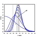 Figure 2
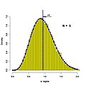 Figure 3
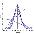 Figure 4
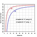 Figure 5


