
User:Talgalili/sandbox/Log transformation (statistics)

In statistics, the log transformation is the application of the logarithmic function to each point in a data set—that is, each data point zi is replaced with the transformed value yi = log(zi). The log transform is usually applied so that the data appear to more closely meet the assumptions of a statistical inference procedure that is to be applied, or to improve the interpretability or appearance of graphs.
The log transform is invertible, and continuous. The transformation is usually applied to a collection of comparable measurements. For example, if we are working with data on peoples' incomes in some currency unit, it would be common to transform each person's income value by the logarithm function.
Motivation
[edit]Guidance for how data should be transformed, or whether a transformation should be applied at all, should come from the particular statistical analysis to be performed. For example, a simple way to construct an approximate 95% confidence interval for the population mean is to take the sample mean plus or minus two standard error units. However, the constant factor 2 used here is particular to the normal distribution, and is only applicable if the sample mean varies approximately normally. The central limit theorem states that in many situations, the sample mean does vary normally if the sample size is reasonably large. However, if the population is substantially skewed and the sample size is at most moderate, the approximation provided by the central limit theorem can be poor, and the resulting confidence interval will likely have the wrong coverage probability. Thus, when there is evidence of substantial skew in the data, it is common to transform the data to a symmetric distribution[1] before constructing a confidence interval. If desired, the confidence interval for some quantile (such as thr median) can then be transformed back to the original scale using exponent, the inverse of the log transformation that was applied to the data.[2][3] it is possible to estimate a quantile using different methods, build a CI for it, and then transform these back to the original scale so to have a CI for the quantile in the original scale. For example, it's possible to estimae the location of the median, after the log transformation, using the arithmetic mean. Then build CI for the median using a CI for the mean and transform the CI back to the original scale using exponent. That transformed CI is then a CI for the median, not the mean.
Data can also be transformed to make them easier to visualize. For example, suppose we have a scatterplot in which the points are the countries of the world, and the data values being plotted are the land area and population of each country. If the plot is made using untransformed data (e.g. square kilometers for area and the number of people for population), most of the countries would be plotted in tight cluster of points in the lower left corner of the graph. The few countries with very large areas and/or populations would be spread thinly around most of the graph's area. Simply rescaling units (e.g., to thousand square kilometers, or to millions of people) will not change this. However, following logarithmic transformations of both area and population, the points will be spread more uniformly in the graph.
Another reason for applying thr log data transformation is to improve interpretability, even if no formal statistical analysis or visualization is to be performed.
In regression
[edit]Data transformation may be used as a remedial measure to make data suitable for modeling with linear regression if the original data violates one or more assumptions of linear regression.[4] For example, the simplest linear regression models assume a linear relationship between the expected value of Y (the response variable to be predicted) and each independent variable (when the other independent variables are held fixed). If linearity fails to hold, even approximately, it is sometimes possible to transform either the independent or dependent variables in the regression model to improve the linearity.[5] For example, addition of quadratic functions of the original independent variables may lead to a linear relationship with expected value of Y, resulting in a polynomial regression model, a special case of linear regression.
Another assumption of linear regression is homoscedasticity, that is the variance of errors must be the same regardless of the values of predictors. If this assumption is violated (i.e. if the data is heteroscedastic), it may be possible to find a transformation of Y alone, or transformations of both X (the predictor variables) and Y, such that the homoscedasticity assumption (in addition to the linearity assumption) holds true on the transformed variables[5] and linear regression may therefore be applied on these.
Yet another application of data transformation is to address the problem of lack of normality in error terms. Univariate normality is not needed for least squares estimates of the regression parameters to be meaningful (see Gauss–Markov theorem). However confidence intervals and hypothesis tests will have better statistical properties if the variables exhibit multivariate normality. Transformations that stabilize the variance of error terms (i.e. those that address heteroscedaticity) often also help make the error terms approximately normal.[5][6]
Examples
[edit]Equation:

- Meaning: A unit increase in X is associated with an average of b units increase in Y.
Equation:

- (From exponentiating both sides of the equation: )
- Meaning: A unit increase in X is associated with an average increase of b units in , or equivalently, Y increases on an average by a multiplicative factor of . For illustrative purposes, if base-10 logarithm were used instead of natural logarithm in the above transformation and the same symbols (a and b) are used to denote the regression coefficients, then a unit increase in X would lead to a times increase in Y on an average. If b were 1, then this implies a 10-fold increase in Y for a unit increase in X


Equation:

- Meaning: A k-fold increase in X is associated with an average of units increase in Y. For illustrative purposes, if base-10 logarithm were used instead of natural logarithm in the above transformation and the same symbols (a and b) are used to denote the regression coefficients, then a tenfold increase in X would result in an average increase of units in Y


Equation:

- (From exponentiating both sides of the equation: )
- Meaning: A k-fold increase in X is associated with a multiplicative increase in Y on an average. Thus if X doubles, it would result in Y changing by a multiplicative factor of .[7]


log log plot
[edit]This article needs additional citations for verification. (December 2009) |

Note the logarithmic scale markings on each of the axes, and that the log x and log y axes (where the logarithms are 0) are where x and y themselves are 1.

In science and engineering, a log–log graph or log–log plot is a two-dimensional graph of numerical data that uses logarithmic scales on both the horizontal and vertical axes. Power functions – relationships of the form – appear as straight lines in a log–log graph, with the exponent corresponding to the slope, and the coefficient corresponding to the intercept. Thus these graphs are very useful for recognizing these relationships and estimating parameters. Any base can be used for the logarithm, though most commonly base 10 (common logs) are used.

The equation for a line on a log–log scale would be:
where m is the slope and b is the intercept point on the log plot.


Slope of a log–log plot
[edit]
To find the slope of the plot, two points are selected on the x-axis, say x1 and x2. Using the above equation: and The slope m is found taking the difference: where F1 is shorthand for F(x1) and F2 is shorthand for F(x2). The figure at right illustrates the formula. Notice that the slope in the example of the figure is negative. The formula also provides a negative slope, as can be seen from the following property of the logarithm:
![{\displaystyle \log[F(x_{1})]=m\log(x_{1})+b,}](https://wikimedia.org/api/rest_v1/media/math/render/svg/101f509699bb7b0432c8b7ae8e649f2d126a9be7)
![{\displaystyle \log[F(x_{2})]=m\log(x_{2})+b.}](https://wikimedia.org/api/rest_v1/media/math/render/svg/4e9241d01657890524140e4bd28935be92a62596)


Log-log linear regression models
[edit]Log–log plots are often use for visualizing log-log linear regression models with (roughly) log-normal, or Log-logistic, errors. In such models, after log-transforming the dependent and independent variables, a Simple linear regression model can be fitted, with the errors becoming homoscedastic. This model is useful when dealing with data that exhibits exponential growth or decay, while the errors continue to grow as the independent value grows (i.e., heteroscedastic error).
As above, in a log-log linear model the relationship between the variables is expressed as a power law. Every unit change in the independent variable will result in a constant percentage change in the dependent variable. The model is expressed as:

Taking the logarithm of both sides, we get:

This is a linear equation in the logarithms of `x` and `y`, with `log(a)` as the intercept and `b` as the slope. In which , and .


Figure 1 illustrates how this looks. It presents two plots generated using 10,000 simulated points. The left plot, titled 'Concave Line with Log-Normal Noise', displays a scatter plot of the observed data (y) against the independent variable (x). The red line represents the 'Median line', while the blue line is the 'Mean line'. This plot illustrates a dataset with a power-law relationship between the variables, represented by a concave line.
When both variables are log-transformed, as shown in the right plot of Figure 1, titled 'Log-Log Linear Line with Normal Noise', the relationship becomes linear. This plot also displays a scatter plot of the observed data against the independent variable, but after both axes are on a logarithmic scale. Here, both the mean and median lines are the same (red) line. This transformation allows us to fit a Simple linear regression model (which can then be transformed back to the original scale - as the median line).

The transformation from the left plot to the right plot in Figure 1 also demonstrates the effect of the log transformation on the distribution of noise in the data. In the left plot, the noise appears to follow a log-normal distribution, which is right-skewed and can be difficult to work with. In the right plot, after the log transformation, the noise appears to follow a normal distribution, which is easier to reason about and model.
This normalization of noise is further analyzed in Figure 2, which presents a line plot of three error metrics (Mean Absolute Error - MAE, Root Mean Square Error - RMSE, and Mean Absolute Logarithmic Error - MALE) calculated over a sliding window of size 28 on the x-axis. The y-axis gives the error, plotted against the independent variable (x). Each error metric is represented by a different color, with the corresponding smoothed line overlaying the original line (since this is just simulated data, the error estimation is a bit jumpy). These error metrics provide a measure of the noise as it varies across different x values.
Log-log linear models are widely used in various fields, including economics, biology, and physics, where many phenomena exhibit power-law behavior. They are also useful in regression analysis when dealing with heteroscedastic data, as the log transformation can help to stabilize the variance.
Common cases
[edit]The logarithm transformation is commonly used for positive data. The power transformation is a family of transformations parameterized by a non-negative value λ that includes the logarithm, square root, and multiplicative inverse transformations as special cases. To approach data transformation systematically, it is possible to use statistical estimation techniques to estimate the parameter λ in the power transformation, thereby identifying the transformation that is approximately the most appropriate in a given setting. Since the power transformation family also includes the identity transformation, this approach can also indicate whether it would be best to analyze the data without a transformation. In regression analysis, this approach is known as the Box–Cox transformation.
A common situation where a data transformation is applied is when a value of interest ranges over several orders of magnitude. Many physical and social phenomena exhibit such behavior — incomes, species populations, galaxy sizes, and rainfall volumes, to name a few. Power transforms, and in particular the logarithm, can often be used to induce symmetry in such data. The logarithm is often favored because it is easy to interpret its result in terms of "fold changes".
The logarithm also has a useful effect on ratios. If we are comparing positive quantities X and Y using the ratio X / Y, then if X < Y, the ratio is in the interval (0,1), whereas if X > Y, the ratio is in the half-line (1,∞), where the ratio of 1 corresponds to equality. In an analysis where X and Y are treated symmetrically, the log-ratio log(X / Y) is zero in the case of equality, and it has the property that if X is K times greater than Y, the log-ratio is the equidistant from zero as in the situation where Y is K times greater than X (the log-ratios are log(K) and −log(K) in these two situations).
Transforming to normality - and log normal distribution
[edit]1. It is not always necessary or desirable to transform a data set to resemble a normal distribution. However, if symmetry or normality are desired, they can often be induced through one of the power transformations.
3. To assess whether normality has been achieved after transformation, any of the standard normality tests may be used. A graphical approach is usually more informative than a formal statistical test and hence a normal quantile plot is commonly used to assess the fit of a data set to a normal population. Alternatively, rules of thumb based on the sample skewness and kurtosis have also been proposed.[8][9]
In probability theory, a log-normal (or lognormal) distribution is a continuous probability distribution of a random variable whose logarithm is normally distributed. Thus, if the random variable X is log-normally distributed, then Y = ln(X) has a normal distribution.[3][10] Equivalently, if Y has a normal distribution, then the exponential function of Y, X = exp(Y) , has a log-normal distribution. A random variable which is log-normally distributed takes only positive real values. It is a convenient and useful model for measurements in exact and engineering sciences, as well as medicine, economics and other topics (e.g., energies, concentrations, lengths, prices of financial instruments, and other metrics).
A log-normal process is the statistical realization of the multiplicative product of many independent random variables, each of which is positive. This is justified by considering the central limit theorem in the log domain (sometimes called Gibrat's law). The log-normal distribution is the maximum entropy probability distribution for a random variate X—for which the mean and variance of ln(X) are specified.[11]
The mode is the point of global maximum of the probability density function. In particular, by solving the equation , we get that:

![{\displaystyle \operatorname {Mode} [X]=e^{\mu -\sigma ^{2}}.}](https://wikimedia.org/api/rest_v1/media/math/render/svg/696ae3ee691abe8666911db6b83228e86d685f85)
Since the log-transformed variable has a normal distribution, and quantiles are preserved under monotonic transformations, the quantiles of are


where is the quantile of the standard normal distribution.

Specifically, the median of a log-normal distribution is equal to its multiplicative mean,[12]
![{\displaystyle \operatorname {Med} [X]=e^{\mu }=\mu ^{*}~.}](https://wikimedia.org/api/rest_v1/media/math/render/svg/2ca3cf66c48a40e98cfbbad81df359a85e2898f5)
Multiple, reciprocal, power
[edit]- Multiplication by a constant: If then for
- Reciprocal: If then
- Power: If then for


Multiplication and division of independent, log-normal random variables
[edit]If two independent, log-normal variables and are multiplied [divided], the product [ratio] is again log-normal, with parameters [] and , where . This is easily generalized to the product of such variables.


More generally, if are independent, log-normally distributed variables, then


Multiplicative central limit theorem
[edit]The geometric or multiplicative mean of independent, identically distributed, positive random variables shows, for , approximately a log-normal distribution with parameters and , assuming is finite.


![{\displaystyle \mu =E[\ln(X_{i})]}](https://wikimedia.org/api/rest_v1/media/math/render/svg/b2a724b374b7dbb96f1b3a40018c88d0011d859e)
![{\displaystyle \sigma ^{2}={\mbox{var}}[\ln(X_{i})]/n}](https://wikimedia.org/api/rest_v1/media/math/render/svg/8cb61e99822586c483b382dd80770ed7df53680d)

In fact, the random variables do not have to be identically distributed. It is enough for the distributions of to all have finite variance and satisfy the other conditions of any of the many variants of the central limit theorem.

This is commonly known as Gibrat's law.
- If is a normal distribution, then
- If is distributed log-normally, then is a normal random variable.
- Let be independent log-normally distributed variables with possibly varying and parameters, and . The distribution of has no closed-form expression, but can be reasonably approximated by another log-normal distribution at the right tail.[13] Its probability density function at the neighborhood of 0 has been characterized[14] and it does not resemble any log-normal distribution. A commonly used approximation due to L.F. Fenton (but previously stated by R.I. Wilkinson and mathematically justified by Marlow[15]) is obtained by matching the mean and variance of another log-normal distribution: In the case that all have the same variance parameter , these formulas simplify to


![{\displaystyle {\begin{aligned}\sigma _{Z}^{2}&=\ln \!\left[{\frac {\sum e^{2\mu _{j}+\sigma _{j}^{2}}(e^{\sigma _{j}^{2}}-1)}{(\sum e^{\mu _{j}+\sigma _{j}^{2}/2})^{2}}}+1\right],\\\mu _{Z}&=\ln \!\left[\sum e^{\mu _{j}+\sigma _{j}^{2}/2}\right]-{\frac {\sigma _{Z}^{2}}{2}}.\end{aligned}}}](https://wikimedia.org/api/rest_v1/media/math/render/svg/4fc943ff6dcd032b6a82e022dd853316e4e77307)


![{\displaystyle {\begin{aligned}\sigma _{Z}^{2}&=\ln \!\left[(e^{\sigma ^{2}}-1){\frac {\sum e^{2\mu _{j}}}{(\sum e^{\mu _{j}})^{2}}}+1\right],\\\mu _{Z}&=\ln \!\left[\sum e^{\mu _{j}}\right]+{\frac {\sigma ^{2}}{2}}-{\frac {\sigma _{Z}^{2}}{2}}.\end{aligned}}}](https://wikimedia.org/api/rest_v1/media/math/render/svg/4e3403a57bdac83cd433bc61aacd2206067d27bc)
For a more accurate approximation, one can use the Monte Carlo method to estimate the cumulative distribution function, the pdf and the right tail.[16][17]
Estimation of parameters
[edit]For determining the maximum likelihood estimators of the log-normal distribution parameters μ and σ, we can use the same procedure as for the normal distribution. Note that where is the density function of the normal distribution . Therefore, the log-likelihood function is


Since the first term is constant with regard to μ and σ, both logarithmic likelihood functions, and , reach their maximum with the same and . Hence, the maximum likelihood estimators are identical to those for a normal distribution for the observations ,


For finite n, the estimator for is unbiased, but the one for is biased. As for the normal distribution, an unbiased estimator for can be obtained by replacing the denominator n by n−1 in the equation for .

When the individual values are not available, but the sample's mean and standard deviation s is, then the Method of moments can be used. The corresponding parameters are determined by the following formulas, obtained from solving the equations for the expectation and variance for and :


![{\displaystyle \operatorname {E} [X]}](https://wikimedia.org/api/rest_v1/media/math/render/svg/44dd294aa33c0865f58e2b1bdaf44ebe911dbf93)
![{\displaystyle \operatorname {Var} [X]}](https://wikimedia.org/api/rest_v1/media/math/render/svg/b79297a808478243e9aab0b27dd1ab583c0f877d)

Interval estimates
[edit]The most efficient way to obtain interval estimates when analyzing log-normally distributed data consists of applying the well-known methods based on the normal distribution to logarithmically transformed data and then to back-transform results if appropriate.
Prediction intervals
[edit]A basic example is given by prediction intervals: For the normal distribution, the interval contains approximately two thirds (68%) of the probability (or of a large sample), and contain 95%. Therefore, for a log-normal distribution, contains 2/3, and contains 95% of the probability. Using estimated parameters, then approximately the same percentages of the data should be contained in these intervals.
![{\displaystyle [\mu -\sigma ,\mu +\sigma ]}](https://wikimedia.org/api/rest_v1/media/math/render/svg/55c87cf54494c57f8aa41a35e60cf1f4ba837fa8)
![{\displaystyle [\mu -2\sigma ,\mu +2\sigma ]}](https://wikimedia.org/api/rest_v1/media/math/render/svg/1cb2f1b03c720b317b0fcf7e012a9bba1a3f418e)
![{\displaystyle [\mu ^{*}/\sigma ^{*},\mu ^{*}\cdot \sigma ^{*}]=[\mu ^{*}{}^{\times }\!\!/\sigma ^{*}]}](https://wikimedia.org/api/rest_v1/media/math/render/svg/90bfe33d3e1ec78fd21196427394f5f4fe5e1836)
![{\displaystyle [\mu ^{*}/(\sigma ^{*})^{2},\mu ^{*}\cdot (\sigma ^{*})^{2}]=[\mu ^{*}{}^{\times }\!\!/(\sigma ^{*})^{2}]}](https://wikimedia.org/api/rest_v1/media/math/render/svg/721c476ec6cdb74bed626ea73e2e5f44bff32d84)
Confidence interval for μ*
[edit]Using the principle, note that a confidence interval for is , where is the standard error and q is the 97.5% quantile of a t distribution with n-1 degrees of freedom. Back-transformation leads to a confidence interval for (the median), is: with
![{\displaystyle [{\widehat {\mu }}\pm q\cdot {\widehat {\mathop {se} }}]}](https://wikimedia.org/api/rest_v1/media/math/render/svg/38626a249b1d579a2af15d2d64ec382789448e60)


![{\displaystyle [{\widehat {\mu }}^{*}{}^{\times }\!\!/(\operatorname {sem} ^{*})^{q}]}](https://wikimedia.org/api/rest_v1/media/math/render/svg/7b9c1579089d540825002f6a247b9991d2d87936)

Confidence interval for μ
[edit]This section needs expansion with: adding the relevant formulas (based on the existing references). You can help by adding to it. (May 2024) |
The literature discusses several options for calculating the confidence interval for (the mean of the log-normal distribution). These include bootstrap as well as various other methods.[18][19]
Notice how it's clear that the expectancy of a log normal distribution is larger than the exponent of the expectancy of the log of log normal r.v., because of Jensen's inequality.
Occurrence and applications
[edit]The log-normal distribution is important in the description of natural phenomena. Many natural growth processes are driven by the accumulation of many small percentage changes which become additive on a log scale. Under appropriate regularity conditions, the distribution of the resulting accumulated changes will be increasingly well approximated by a log-normal, as noted in the section above on "Multiplicative Central Limit Theorem". This is also known as Gibrat's law, after Robert Gibrat (1904–1980) who formulated it for companies.[20] If the rate of accumulation of these small changes does not vary over time, growth becomes independent of size. Even if this assumption is not true, the size distributions at any age of things that grow over time tends to be log-normal.[citation needed] Consequently, reference ranges for measurements in healthy individuals are more accurately estimated by assuming a log-normal distribution than by assuming a symmetric distribution about the mean.[citation needed]
A second justification is based on the observation that fundamental natural laws imply multiplications and divisions of positive variables. Examples are the simple gravitation law connecting masses and distance with the resulting force, or the formula for equilibrium concentrations of chemicals in a solution that connects concentrations of educts and products. Assuming log-normal distributions of the variables involved leads to consistent models in these cases.
Specific examples are given in the following subsections.[5] contains a review and table of log-normal distributions from geology, biology, medicine, food, ecology, and other areas.[21] is a review article on log-normal distributions in neuroscience, with annotated bibliography.
Human behavior
[edit]- The length of comments posted in Internet discussion forums follows a log-normal distribution.[22]
- Users' dwell time on online articles (jokes, news etc.) follows a log-normal distribution.[23]
- The length of chess games tends to follow a log-normal distribution.[24]
- Onset durations of acoustic comparison stimuli that are matched to a standard stimulus follow a log-normal distribution.[25]
Biology and medicine
[edit]- Measures of size of living tissue (length, skin area, weight).[26]
- Incubation period of diseases.[27]
- Diameters of banana leaf spots, powdery mildew on barley.[5]
- For highly communicable epidemics, such as SARS in 2003, if public intervention control policies are involved, the number of hospitalized cases is shown to satisfy the log-normal distribution with no free parameters if an entropy is assumed and the standard deviation is determined by the principle of maximum rate of entropy production.[28]
- The length of inert appendages (hair, claws, nails, teeth) of biological specimens, in the direction of growth.[citation needed]
- The normalised RNA-Seq readcount for any genomic region can be well approximated by log-normal distribution.
- The PacBio sequencing read length follows a log-normal distribution.[29]
- Certain physiological measurements, such as blood pressure of adult humans (after separation on male/female subpopulations).[30]
- Several pharmacokinetic variables, such as Cmax, elimination half-life and the elimination rate constant.[31]
- In neuroscience, the distribution of firing rates across a population of neurons is often approximately log-normal. This has been first observed in the cortex and striatum [32] and later in hippocampus and entorhinal cortex,[33] and elsewhere in the brain.[21][34] Also, intrinsic gain distributions and synaptic weight distributions appear to be log-normal[35] as well.
- Neuron densities in the cerebral cortex, due to the noisy cell division process during neurodevelopment.[36]
- In operating-rooms management, the distribution of surgery duration.
- In the size of avalanches of fractures in the cytoskeleton of living cells, showing log-normal distributions, with significantly higher size in cancer cells than healthy ones.[37]
Chemistry
[edit]- Particle size distributions and molar mass distributions.
- The concentration of rare elements in minerals.[38]
- Diameters of crystals in ice cream, oil drops in mayonnaise, pores in cocoa press cake.[5]
Hydrology
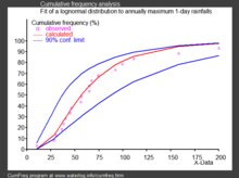
[edit]- In hydrology, the log-normal distribution is used to analyze extreme values of such variables as monthly and annual maximum values of daily rainfall and river discharge volumes.[39]
- The image on the right, made with CumFreq, illustrates an example of fitting the log-normal distribution to ranked annually maximum one-day rainfalls showing also the 90% confidence belt based on the binomial distribution.[40]
- The rainfall data are represented by plotting positions as part of a cumulative frequency analysis.
Social sciences and demographics
[edit]- In economics, there is evidence that the income of 97%–99% of the population is distributed log-normally.[41] (The distribution of higher-income individuals follows a Pareto distribution).[42]
- If an income distribution follows a log-normal distribution with standard deviation , then the Gini coefficient, commonly use to evaluate income inequality, can be computed as where is the error function, since , where is the cumulative distribution function of a standard normal distribution.
- In finance, in particular the Black–Scholes model, changes in the logarithm of exchange rates, price indices, and stock market indices are assumed normal[43] (these variables behave like compound interest, not like simple interest, and so are multiplicative). However, some mathematicians such as Benoit Mandelbrot have argued [44] that log-Lévy distributions, which possesses heavy tails would be a more appropriate model, in particular for the analysis for stock market crashes. Indeed, stock price distributions typically exhibit a fat tail.[45] The fat tailed distribution of changes during stock market crashes invalidate the assumptions of the central limit theorem.
- In scientometrics, the number of citations to journal articles and patents follows a discrete log-normal distribution.[46][47]
- City sizes (population) satisfy Gibrat's Law.[48] The growth process of city sizes is proportionate and invariant with respect to size. From the central limit theorem therefore, the log of city size is normally distributed.
- The number of sexual partners appears to be best described by a log-normal distribution.[49]


Technology
[edit]- In reliability analysis, the log-normal distribution is often used to model times to repair a maintainable system.[50]
- In wireless communication, "the local-mean power expressed in logarithmic values, such as dB or neper, has a normal (i.e., Gaussian) distribution."[51] Also, the random obstruction of radio signals due to large buildings and hills, called shadowing, is often modeled as a log-normal distribution.
- Particle size distributions produced by comminution with random impacts, such as in ball milling.[52]
- The file size distribution of publicly available audio and video data files (MIME types) follows a log-normal distribution over five orders of magnitude.[53]
- File sizes of 140 million files on personal computers running the Windows OS, collected in 1999.[54][22]
- Sizes of text-based emails (1990s) and multimedia-based emails (2000s).[22]
- In computer networks and Internet traffic analysis, log-normal is shown as a good statistical model to represent the amount of traffic per unit time. This has been shown by applying a robust statistical approach on a large groups of real Internet traces. In this context, the log-normal distribution has shown a good performance in two main use cases: (1) predicting the proportion of time traffic will exceed a given level (for service level agreement or link capacity estimation) i.e. link dimensioning based on bandwidth provisioning and (2) predicting 95th percentile pricing.[55]
- in physical testing when the test produces a time-to-failure of an item under specified conditions, the data is often best analyzed using a lognormal distribution.[56][57]
Variance stabilizing transformations
[edit]The aim behind the choice of a variance-stabilizing transformation is to find a simple function ƒ to apply to values x in a data set to create new values y = ƒ(x) such that the variability of the values y is not related to their mean value.
Many types of statistical data exhibit a "variance-on-mean relationship", meaning that the variability is different for data values with different expected values. As an example, in comparing different populations in the world, the variance of income tends to increase with mean income. If we consider a number of small area units (e.g., counties in the United States) and obtain the mean and variance of incomes within each county, it is common that the counties with higher mean income also have higher variances.
A variance-stabilizing transformation aims to remove a variance-on-mean relationship, so that the variance becomes constant relative to the mean.
Example: relative variance
[edit]If X is a positive random variable and for some constant, s, the variance is given as h(μ) = s2μ2 then the standard deviation is proportional to the mean, which is called fixed relative error. In this case, the variance-stabilizing transformation is

That is, the variance-stabilizing transformation is the logarithmic transformation.
Relationship to the delta method
[edit]Here, the delta method is presented in a rough way, but it is enough to see the relation with the variance-stabilizing transformations. To see a more formal approach see delta method.
Let be a random variable, with and . Define , where is a regular function. A first order Taylor approximation for is:
![{\displaystyle E[X]=\mu }](https://wikimedia.org/api/rest_v1/media/math/render/svg/51ed977b56d8e513d9eb92193de5454ac545231e)


From the equation above, we obtain:
- and
![{\displaystyle E[Y]\approx g(\mu )}](https://wikimedia.org/api/rest_v1/media/math/render/svg/9350eb857fea07cb25e9dd073a6305e754a15fd4)
![{\displaystyle \operatorname {Var} [Y]\approx \sigma ^{2}g'(\mu )^{2}}](https://wikimedia.org/api/rest_v1/media/math/render/svg/dc73d0925a27f157089c24ac4f0c8279500d4271)
This approximation method is called delta method.
See also
[edit]MAIN sources:
- Data transformation (statistics)
- Log-normal distribution
- Log–log plot
- Variance-stabilizing transformation
- Box–Cox distribution
- Power transform
- Logarithm
- Logarithmic scale
- Delta method (for exp of approx normal distributions)
- Median test
TODO: (edit)
- Arcsin
- Feature engineering
- Logit
- Nonlinear regression § Transformation
- Pearson correlation coefficient
- Power transform (Box–Cox)
- Wilson–Hilferty transformation
- Whitening transformation
References
[edit]- ^ Kuhn, Max; Johnson, Kjell (2013). Applied predictive modeling. New York. doi:10.1007/978-1-4614-6849-3. ISBN 9781461468493. LCCN 2013933452. OCLC 844349710. S2CID 60246745.
{{cite book}}: CS1 maint: location missing publisher (link) - ^ Altman, Douglas G.; Bland, J. Martin (1996-04-27). "Statistics notes: Transformations, means, and confidence intervals". BMJ. 312 (7038): 1079. doi:10.1136/bmj.312.7038.1079. ISSN 0959-8138. PMC 2350916. PMID 8616417.
- ^ a b "Data transformations - Handbook of Biological Statistics". www.biostathandbook.com. Retrieved 2019-03-19. Cite error: The named reference ":1" was defined multiple times with different content (see the help page).
- ^ "Lesson 9: Data Transformations | STAT 501". newonlinecourses.science.psu.edu. Retrieved 2019-03-17.
- ^ a b c d e f Kutner, Michael H.; Nachtsheim, Christopher J.; Neter, John; Li, William (2005). Applied linear statistical models (5th ed.). Boston: McGraw-Hill Irwin. pp. 129–133. ISBN 0072386886. LCCN 2004052447. OCLC 55502728. Cite error: The named reference ":0" was defined multiple times with different content (see the help page).
- ^ Altman, Douglas G.; Bland, J. Martin (1996-03-23). "Statistics Notes: Transforming data". BMJ. 312 (7033): 770. doi:10.1136/bmj.312.7033.770. ISSN 0959-8138. PMC 2350481. PMID 8605469.
- ^ "9.3 - Log-transforming Both the Predictor and Response | STAT 501". newonlinecourses.science.psu.edu. Retrieved 2019-03-17.
- ^ Kim, Hae-Young (2013-02-01). "Statistical notes for clinical researchers: assessing normal distribution (2) using skewness and kurtosis". Restorative Dentistry & Endodontics. 38 (1): 52–54. doi:10.5395/rde.2013.38.1.52. ISSN 2234-7658. PMC 3591587. PMID 23495371.
- ^ "Testing normality including skewness and kurtosis". imaging.mrc-cbu.cam.ac.uk. Retrieved 2019-03-18.
- ^ "1.3.6.6.9. Lognormal Distribution". www.itl.nist.gov. U.S. National Institute of Standards and Technology (NIST). Retrieved 2020-09-13.
- ^ Park, Sung Y.; Bera, Anil K. (2009). "Maximum entropy autoregressive conditional heteroskedasticity model" (PDF). Journal of Econometrics. 150 (2): 219–230, esp. Table 1, p. 221. CiteSeerX 10.1.1.511.9750. doi:10.1016/j.jeconom.2008.12.014. Archived from the original (PDF) on 2016-03-07. Retrieved 2011-06-02.
- ^ Daly, Leslie E.; Bourke, Geoffrey Joseph (2000). Interpretation and Uses of Medical Statistics (5th ed.). Oxford, UK: Wiley-Blackwell. p. 89. doi:10.1002/9780470696750. ISBN 978-0-632-04763-5. PMC 1059583; print edition. Online eBook ISBN 9780470696750
- ^ Asmussen, S.; Rojas-Nandayapa, L. (2008). "Asymptotics of Sums of Lognormal Random Variables with Gaussian Copula" (PDF). Statistics and Probability Letters. 78 (16): 2709–2714. doi:10.1016/j.spl.2008.03.035.
- ^ Cite error: The named reference
Gaowas invoked but never defined (see the help page). - ^ Marlow, NA. (Nov 1967). "A normal limit theorem for power sums of independent normal random variables". Bell System Technical Journal. 46 (9): 2081–2089. doi:10.1002/j.1538-7305.1967.tb04244.x.
- ^ Botev, Z. I.; L'Ecuyer, P. (2017). "Accurate computation of the right tail of the sum of dependent log-normal variates". 2017 Winter Simulation Conference (WSC), 3rd–6th Dec 2017. Las Vegas, NV, USA: IEEE. pp. 1880–1890. arXiv:1705.03196. doi:10.1109/WSC.2017.8247924. ISBN 978-1-5386-3428-8.
- ^ Asmussen, A.; Goffard, P.-O.; Laub, P. J. (2016). "Orthonormal polynomial expansions and lognormal sum densities". arXiv:1601.01763v1 [math.PR].
- ^ Olsson, Ulf. "Confidence intervals for the mean of a log-normal distribution." Journal of Statistics Education 13.1 (2005).pdf html
- ^ user10525, How do I calculate a confidence interval for the mean of a log-normal data set?, URL (version: 2022-12-18): https://stats.stackexchange.com/q/33395
- ^ Sutton, John (Mar 1997). "Gibrat's Legacy". Journal of Economic Literature. 32 (1): 40–59. JSTOR 2729692.
- ^ a b Buzsáki, György; Mizuseki, Kenji (2017-01-06). "The log-dynamic brain: how skewed distributions affect network operations". Nature Reviews. Neuroscience. 15 (4): 264–278. doi:10.1038/nrn3687. ISSN 1471-003X. PMC 4051294. PMID 24569488.
- ^ a b c Pawel, Sobkowicz; et al. (2013). "Lognormal distributions of user post lengths in Internet discussions - a consequence of the Weber-Fechner law?". EPJ Data Science.
- ^ Yin, Peifeng; Luo, Ping; Lee, Wang-Chien; Wang, Min (2013). Silence is also evidence: interpreting dwell time for recommendation from psychological perspective. ACM International Conference on KDD.
- ^ "What is the average length of a game of chess?". chess.stackexchange.com. Retrieved 14 April 2018.
- ^ Cite error: The named reference
Acoustic Stimuli Revisited 2016was invoked but never defined (see the help page). - ^ Huxley, Julian S. (1932). Problems of relative growth. London. ISBN 978-0-486-61114-3. OCLC 476909537.
- ^ Sartwell, Philip E. "The distribution of incubation periods of infectious disease." American journal of hygiene 51 (1950): 310-318.
- ^ S. K. Chan, Jennifer; Yu, Philip L. H. (2006). "Modelling SARS data using threshold geometric process". Statistics in Medicine. 25 (11): 1826–1839. doi:10.1002/sim.2376. PMID 16345017. S2CID 46599163.
- ^ Ono, Yukiteru; Asai, Kiyoshi; Hamada, Michiaki (2013-01-01). "PBSIM: PacBio reads simulator—toward accurate genome assembly". Bioinformatics. 29 (1): 119–121. doi:10.1093/bioinformatics/bts649. ISSN 1367-4803. PMID 23129296.
- ^ Makuch, Robert W.; D.H. Freeman; M.F. Johnson (1979). "Justification for the lognormal distribution as a model for blood pressure". Journal of Chronic Diseases. 32 (3): 245–250. doi:10.1016/0021-9681(79)90070-5. PMID 429469.
- ^ Lacey, L. F.; Keene, O. N.; Pritchard, J. F.; Bye, A. (1997-01-01). "Common noncompartmental pharmacokinetic variables: are they normally or log-normally distributed?". Journal of Biopharmaceutical Statistics. 7 (1): 171–178. doi:10.1080/10543409708835177. ISSN 1054-3406. PMID 9056596.
- ^ Scheler, Gabriele; Schumann, Johann (2006-10-08). Diversity and stability in neuronal output rates. 36th Society for Neuroscience Meeting, Atlanta.
- ^ Mizuseki, Kenji; Buzsáki, György (2013-09-12). "Preconfigured, skewed distribution of firing rates in the hippocampus and entorhinal cortex". Cell Reports. 4 (5): 1010–1021. doi:10.1016/j.celrep.2013.07.039. ISSN 2211-1247. PMC 3804159. PMID 23994479.
- ^ Wohrer, Adrien; Humphries, Mark D.; Machens, Christian K. (2013-04-01). "Population-wide distributions of neural activity during perceptual decision-making". Progress in Neurobiology. 103: 156–193. doi:10.1016/j.pneurobio.2012.09.004. ISSN 1873-5118. PMC 5985929. PMID 23123501.
- ^ Scheler, Gabriele (2017-07-28). "Logarithmic distributions prove that intrinsic learning is Hebbian". F1000Research. 6: 1222. doi:10.12688/f1000research.12130.2. PMC 5639933. PMID 29071065.
- ^ Morales-Gregorio, Aitor; van Meegen, Alexander; van Albada, Sacha (2023). "Ubiquitous lognormal distribution of neuron densities in mammalian cerebral cortex". Cerebral Cortex. 33 (16): 9439–9449. doi:10.1093/cercor/bhad160. PMC 10438924. PMID 37409647.
- ^ Polizzi, Stefano; Laperrousaz, Bastien; Perez-Reche, Francisco J; Nicolini, Franck E; Satta, Véronique Maguer; Arneodo, Alain; Argoul, Françoise (2018-05-29). "A minimal rupture cascade model for living cell plasticity". New Journal of Physics. 20 (5): 053057. doi:10.1088/1367-2630/aac3c7. hdl:2164/10561. ISSN 1367-2630.
- ^ Ahrens, L. H. (1954-02-01). "The lognormal distribution of the elements (A fundamental law of geochemistry and its subsidiary)". Geochimica et Cosmochimica Acta. 5 (2): 49–73. Bibcode:1954GeCoA...5...49A. doi:10.1016/0016-7037(54)90040-X. ISSN 0016-7037.
- ^ Oosterbaan, R.J. (1994). "6: Frequency and Regression Analysis" (PDF). In Ritzema, H.P. (ed.). Drainage Principles and Applications, Publication 16. Wageningen, The Netherlands: International Institute for Land Reclamation and Improvement (ILRI). pp. 175–224. ISBN 978-90-70754-33-4.
- ^ CumFreq, free software for distribution fitting
- ^ Clementi, Fabio; Gallegati, Mauro (2005) "Pareto's law of income distribution: Evidence for Germany, the United Kingdom, and the United States", EconWPA
- ^ Wataru, Souma (2002-02-22). "Physics of Personal Income". In Takayasu, Hideki (ed.). Empirical Science of Financial Fluctuations: The Advent of Econophysics. Springer. arXiv:cond-mat/0202388. doi:10.1007/978-4-431-66993-7.
- ^ Black, F.; Scholes, M. (1973). "The Pricing of Options and Corporate Liabilities". Journal of Political Economy. 81 (3): 637. doi:10.1086/260062. S2CID 154552078.
- ^ Mandelbrot, Benoit (2004). The (mis-)Behaviour of Markets. Basic Books. ISBN 9780465043552.
- ^ Bunchen, P., Advanced Option Pricing, University of Sydney coursebook, 2007
- ^ Thelwall, Mike; Wilson, Paul (2014). "Regression for citation data: An evaluation of different methods". Journal of Informetrics. 8 (4): 963–971. arXiv:1510.08877. doi:10.1016/j.joi.2014.09.011. S2CID 8338485.
- ^ Sheridan, Paul; Onodera, Taku (2020). "A Preferential Attachment Paradox: How Preferential Attachment Combines with Growth to Produce Networks with Log-normal In-degree Distributions". Scientific Reports. 8 (1): 2811. arXiv:1703.06645. doi:10.1038/s41598-018-21133-2. PMC 5809396. PMID 29434232.
- ^ Eeckhout, Jan (2004). "Gibrat's Law for (All) Cities". American Economic Review. 94 (5): 1429–1451. doi:10.1257/0002828043052303. JSTOR 3592829 – via JSTOR.
- ^ Kault, David (1996). "The Shape of the Distribution of the Number of Sexual Partners". Statistics in Medicine. 15 (2): 221–230. doi:10.1002/(SICI)1097-0258(19960130)15:2<221::AID-SIM148>3.0.CO;2-Q. PMID 8614756.
- ^ O'Connor, Patrick; Kleyner, Andre (2011). Practical Reliability Engineering. John Wiley & Sons. p. 35. ISBN 978-0-470-97982-2.
- ^ "Shadowing". www.WirelessCommunication.NL. Archived from the original on January 13, 2012.
- ^ Dexter, A. R.; Tanner, D. W. (July 1972). "Packing Densities of Mixtures of Spheres with Log-normal Size Distributions". Nature Physical Science. 238 (80): 31–32. Bibcode:1972NPhS..238...31D. doi:10.1038/physci238031a0. ISSN 2058-1106.
- ^ Gros, C; Kaczor, G.; Markovic, D (2012). "Neuropsychological constraints to human data production on a global scale". The European Physical Journal B. 85 (28): 28. arXiv:1111.6849. Bibcode:2012EPJB...85...28G. doi:10.1140/epjb/e2011-20581-3. S2CID 17404692.
- ^ Douceur, John R.; Bolosky, William J. (1999-05-01). "A large-scale study of file-system contents". ACM SIGMETRICS Performance Evaluation Review. 27 (1): 59–70. doi:10.1145/301464.301480. ISSN 0163-5999.
- ^ Alamsar, Mohammed; Parisis, George; Clegg, Richard; Zakhleniuk, Nickolay (2019). "On the Distribution of Traffic Volumes in the Internet and its Implications". arXiv:1902.03853 [cs.NI].
- ^ ASTM D3654, Standard Test Method for Shear Adhesion on Pressure-Sensitive Tapesw
- ^ ASTM D4577, Standard Test Method for Compression Resistance of a container Under Constant Load>\
External links
[edit]- Log Transformations for Skewed and Wide Distributions – discussing the log and the "signed logarithm" transformations (A chapter from "Practical Data Science with R").